Terminal Value in DCF: Formula, Methods & Interview Questions

The Discounted Cash Flow (DCF) model is one of the most widely used valuation methods in finance, and you are almost guaranteed to face questions about it during investment banking interviews. It is built on the premise that a company is worth the sum of all its future free cash flows, discounted back to today's value. 

But it's not possible to reliably forecast cash flows year-by-year forever. To solve this without ignoring the company's long-term worth, DCF models forecast in detail for a few years within the explicit forecast period or projection period. Then they bundle everything beyond that forecast horizon into a single figure known as terminal value in DCF.

This comprehensive guide breaks down why terminal value is important in DCF, how it's calculated using the perpetuity growth model vs exit multiple model, how it affects implied enterprise value, common DCF terminal value mistakes, and typical terminal value interview questions.

What Is Terminal Value?

Terminal value is the estimated present value of a company’s cash flows beyond the explicit forecast period, assuming the business operates indefinitely. To capture this infinite timeline, finance professionals structure the valuation as a two-stage DCF model:

• Stage 1 - The Forecast Period (Years 1–10): Also called the projection period or forecast horizon, this is the near-term timeframe where you project detailed, year-by-year free cash flow (FCF) / unlevered free cash flow (UFCF) based on specific growth and margin assumptions.
• Stage 2 - The Terminal Period (Year 11+ to Infinity): Begins after Stage 1 ends and lasts into infinity where detailed forecasting becomes unreliable. It assumes the company has matured to predictable cash flows and will grow at a steady, sustainable rate. So you normalize or adjust the forecast period’s final year cash flows to reflect that. Then the normalized figure acts as a stable starting point to which you can apply terminal value formulas that bundle all remaining infinite cash flows into a single sum.

Without calculating DCF terminal value, a model would imply the company abruptly ceases to exist after the forecast period. Hence it would fail to capture a business’s true intrinsic value.

Why Is Terminal Value Important in a DCF?

Beyond helping capture a business’s intrinsic value, terminal value is important in a DCF because of how much it drives the final number. It usually accounts for 60% to 80% of a company's total value, making its accuracy highly influential to the final DCF outcome. The reason it makes up much of the valuation figure is that terminal value captures decades of future cash flows while the forecast period only covers a few years.

That weight also makes terminal value the most sensitive part of the DCF model. A tiny adjustment to the assumptions used in calculating terminal value, like the discount rate, can change the final enterprise value by millions.

How to Calculate Terminal Value in DCF

For the terminal value calculations, there are two standard methods used and interviewers expect you to understand and compare both.

The first is the Perpetuity Growth Method, which assumes the company will grow its Free Cash Flow (FCF) at a constant, sustainable rate forever. The second is the Exit Multiple Method, which assumes the company is sold at the end of the forecast period for a valuation multiple common in the current market.

Perpetuity Growth Method

This method, also called the growth in perpetuity approach, treats the company's cash flows like a perpetuity, meaning an infinite stream of cash flows growing at a fixed rate forever. The formula is derived from the Gordon Growth Model.

When using the perpetuity growth method, the terminal value formula DCF analysts use is:

Where:

• FCFₙ = Final year FCF or normalized cash flow in the final year of your forecast period
• g = Perpetuity growth rate, also called the terminal growth rate, or the constant growth rate the company grows at, forever, after the forecast period
• r = Discount rate (typically the Weighted Average Cost of Capital, or WACC)

Essentially, you’re taking the normalized final year's free cash flow, growing it one more year to get the first year of the perpetuity period, and then dividing by the difference between WACC and g. That denominator is the most critical piece of the equation. A wider gap between the discount rate and the growth rate shrinks the terminal value, while a narrower one increases it dramatically.

When applying this terminal value formula, the chosen constant growth rate is highly sensitive. It should never exceed the long-term economic growth rate (GDP growth), as no company can grow faster than the economy forever. Typically, it is set between the rate of consumer inflation and GDP growth (2% to 4%).

Exit Multiple Method

Instead of assuming infinite operations, the Exit Multiple Method assumes the company is sold at the end of the forecast period. You value that hypothetical sale by applying a valuation multiple common in the current market to a final-year financial metric.

The terminal value formula for this approach is:

The most common financial metric used is EBITDA, which is then multiplied by an EV/EBITDA multiple. Analysts find a justifiable exit multiple by looking at trading multiples of comparable companies (Comps) and pricing benchmarks from recent M&A deals or precedent transactions.

Perpetuity Growth Method vs. Exit Multiple Method

Both the perpetuity growth and exit multiple methods answer the same question, but they lean on different assumptions.

The perpetuity growth method is rooted in fundamentals which makes it more theoretically pure, since it doesn't rely on market pricing or comparable companies. But its weakness is sensitivity. Small changes in the growth rate or discount rate can swing terminal value significantly, which makes the output easy to manipulate, intentionally or not. It's best suited for mature, stable businesses with predictable cash flows, or situations where comparable market data is limited.

For the exit multiple method, the focus is market reality rather than fundamentals. Its key advantage is that it shows what buyers are actually paying for similar businesses today, making it highly defensible to investment committees. But its major weakness is cyclicality. Using a current multiple assumes today's market conditions will exist a decade from now, ignoring the risk of future economic downturns, shifts in investment sentiment, or multiple compression. It's best suited for transaction-oriented valuations like M&A and private equity, or situations where you need defensible, market-based assumptions.

In practice though, most analysts calculate terminal value using both methods and compare the results. Or, they add a cross-checking terminal value step where they find what the implied growth rate or implied exit multiple each method would need to produce the other method's answer. If the two numbers are wildly different, then something is off. Either the growth rate assumption is too aggressive, or the exit multiple doesn't reflect the company's true growth trajectory. 

How Terminal Value Affects Enterprise Value

Once you've calculated terminal value using either formula, you must discount it back to the present, just like every other cash flow in the forecast period. This is due to the time value of money which means cash in the future is worth less than money today. 

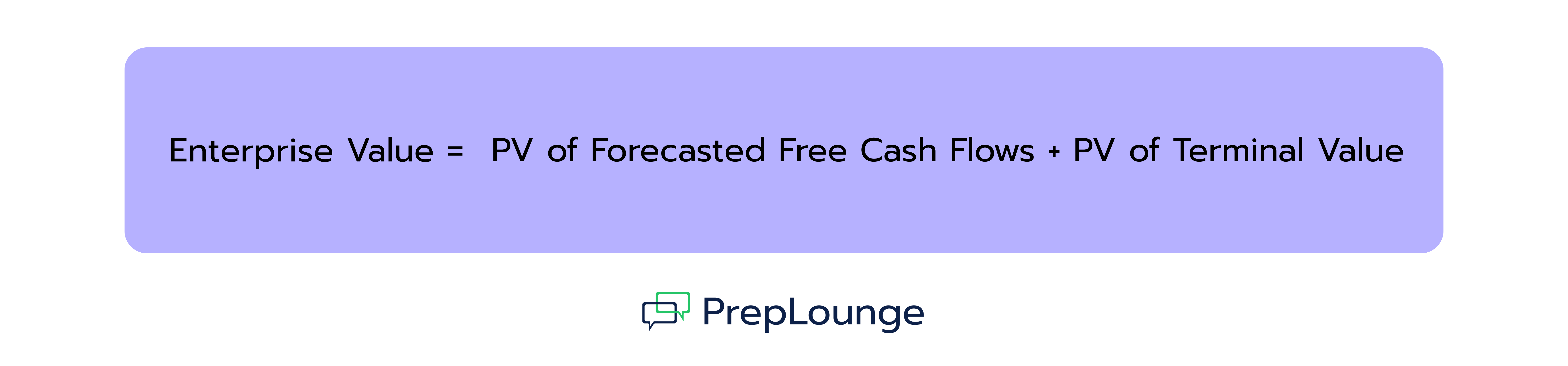
To find the present value of terminal value, discount it using the WACC (Weighted Average Cost of Capital) over the number of years in your forecast period. Then add it to the near term cash flows to find the enterprise value.

The formula for enterprise value is:

Where: PV is present value

Even after heavy discounting, this single present value terminal value figure will still heavily dictate the implied enterprise value.

Terminal Value Calculation Example

Let’s say you want to find the terminal value of a company with the following at the end of year 5, which is the final year of your forecast period:

• Final year free cash flow (FCF) / unlevered free cash flow (UFCF): $100 million
• WACC (Weighted Average Cost of Capital): 10%
• Perpetuity growth rate / terminal growth rate (g): 3%
• Final year EBITDA: $150 million
• EV/EBITDA multiple from comparable companies (Comps): 8x

Using the Perpetuity Growth Method:

Using the Exit Multiple Method:

The two methods land in a similar ballpark of $1,471 million vs. $1,200 million. To finish the calculation for your implied enterprise value, you must find the present value of terminal value (PV of TV). Using the perpetuity growth result as an example:

This $913.64 million is then added directly to the present value of your year 1–5 cash flows to determine the total intrinsic value of the business.

Common Mistakes When Calculating Terminal Value 

Here are the most common DCF terminal value mistakes and how to avoid them.

• Mismatched Multiples: You must pair Enterprise Value (EV) multiples with pre-debt metrics, like EBITDA, EBIT, or Revenue, and Equity Value multiples with post-debt metrics, like Net Income or P/E. Mixing them breaks the capital structure logic of your model because you’d be comparing cash flows belonging to all investors against values belonging only to shareholders.
• Aggressive Growth Rates: Setting a perpetual growth rate at four or five percent because a company is currently performing well is unrealistic. This rate lasts for eternity, meaning it cannot logically exceed long-term GDP growth.
• Double Counting Final Forecast Year: The perpetuity growth formula requires next year's cash flow, not the final forecasted year's cash flow. The growth adjustment in the numerator solves that and skipping it is a frequent error that understates terminal value.
• Using an Un-Normalized Final Year: Plugging in the final forecast year's raw FCF without adjusting for one-off items like a tax break, a lawsuit settlement, or unusually low capex, brings that distortion into an assumption that's meant to repeat forever. An inflated final year overstates terminal value while a depressed one understates it.
• Ignoring Cross Checks: Relying on only one calculation method without a terminal value sensitivity analysis or sanity-checking it against the other prevents you from catching unreasonable assumptions before they skew your valuation.
• Forgetting to Discount: Terminal value is calculated as of the final forecast year, not today. Adding the raw terminal value directly to your enterprise value equation without discounting it back to Year 0 will massively overstate the company's worth considering the time value of money.

Typical Terminal Value Interview Questions

The most common terminal value interview questions test your ability to choose the right calculation method, justify your growth and discount rate assumptions, and cross-check valuation assumptions. So, expect to answer questions on perpetuity growth vs. exit multiple trade-offs, calculating implied growth rates, the impact of changing discount rates (WACC), and standardizing cash flows to reflect a mature steady state.

Here are a few sample questions for your practice.

1. How do you check if your Exit Multiple makes sense?

You should perform a sanity check by cross-checking terminal value numbers. You can back-solve for the implied terminal growth rate using the Gordon Growth formula. If your chosen exit multiple yields an implied growth rate that is significantly higher than long-term GDP growth, your multiple is too aggressive and needs to be adjusted downward.

2. What happens to the Terminal Value if the WACC increases?

If the discount rate (WACC) increases, the terminal value will decrease. WACC is in the denominator of the valuation formula. A higher discount rate increases the denominator, which reduces both the raw terminal value and the present value of terminal value when discounted back to today.

3. What's the difference between the perpetuity growth method and the exit multiple method? 

The perpetuity growth method is purely fundamental and intrinsic. It assumes the business will operate as a steady-state perpetuity forever. The exit multiple method is market-driven and assumes the business will be valued based on what comparable companies (Comps) and precedent transactions dictate in the open market today.

Conclusion

Mastering how to calculate terminal value is non-negotiable for financial modeling and acing technical finance interviews. Terminal value makes up a majority of an enterprise value, specifically about 60-80%. So, minor adjustments to the perpetuity growth rate or trading multiples create massive ripple effects. Always utilize a thorough sensitivity analysis and run appropriate cross-checks to ensure your valuation stands up to professional scrutiny.

To ace technical IB interviews, master the two terminal value formulas, understand why the numbers move the way they do, and be prepared to catch the mistakes that quietly distort them. 

Here Are More Interesting Articles!